Credit Scorecard Model Report - 3_Scoring_v28_before

Executive Summary

Model

Model Type

Logistic Regression with WOE-transformed features

Eval

Model Evaluated

2 Methods with different class balancing techniques

Feat

Features Used

7 WOE-binned predictive features

Score

Scoring Methods

Method 1: WOE Points | Method 2: Probability-to-Score

                    Key Findings
                    Top Predictive Features: Interest Burden, Out Prncp Inv, and Total Pymnt
                            Inv
Model Stability: PSI analysis shows stable distributions across time
                            windows
SHAP Validation: All 2 approaches for class balancing techniques show
                            consistent feature importance rankings
Both Methods Compliant: Method 1 (bin-based) excels at transparency for
                            consumer explanations; Method 2 (probability-based) provides continuous scoring for
                            portfolio analytics
Score Differences Expected: Both methods use the same model but different
                            scaling.

                

Model Performance Metrics

Note: The following metrics summarize the classification performance of the underlying logistic regression model. Both scoring methods (Method 1 and Method 2) use the same model, so these metrics apply to both.

Model Discrimination

Good

AUC_ROC: 0.88

AUC_PR: 0.974

GINI: 0.759

Max. KS: 0.617

Population Stability

Stable

PSI < 0.1 across windows

Feature Quality

Strong

7 WOE-binned features

Classification Performance Overview

The model demonstrates strong discriminatory power in separating good from bad credits. Key performance indicators include:

AUC-ROC: Measures the model's ability to rank borrowers correctly
AUC-PR: It summarizes the trade-off between precision and recall across different classification thresholds. It is sensitive to class prevalence and should be interpreted jointly with KS and ROC
Accuracy: Overall percentage of correct classifications
Precision & Recall: Trade-off between false positives and false negatives
PSI: Population stability across different time periods

Interpretation Guidelines

AUC >= 0.75: Good discrimination
PSI < 0.1: Stable population (low drift)
PSI 0.1-0.2: Moderate drift - monitor closely
PSI >= 0.2: Significant drift - model recalibration may be needed

Pre-Selected Features (statsmodels):

Statistical significance of model coefficients. Features with P-Value greater than 0.05 may not be statistically significant.

Feature	Coefficient	P_Value	Std_Error	Z_Score
const	3.242278	0.0000e+00	0.014299	226.744967
WOE_interest_burden_bin	2.359639	0.0000e+00	0.021001	112.356356
WOE_total_pymnt_inv_bin	1.953125	0.0000e+00	0.018349	106.442047
WOE_out_prncp_inv_bin	1.532761	0.0000e+00	0.015491	98.944325
WOE_pymnt_per_account_bin	1.259167	0.0000e+00	0.015760	79.893927
WOE_annual_inc_bin	-1.132092	0.0000e+00	0.014955	-75.701271
WOE_total_rec_int_bin	-0.648790	0.0000e+00	0.014012	-46.303156
WOE_int_rate_bin	-0.514660	2.3339e-269	0.014677	-35.064628
WOE_credit_stress_index_bin	0.304132	1.2746e-78	0.016201	18.772214
WOE_mths_since_issue_d_bin	0.282676	2.3575e-90	0.014024	20.156552
WOE_loan_concentration_bin	0.256821	7.3746e-93	0.012565	20.439996
WOE_dti_with_loan_bin	-0.224815	1.4492e-77	0.012059	-18.642637
WOE_term_bin	-0.161864	1.1718e-38	0.012448	-13.003297
WOE_available_credit_pct_bnetli	-0.155586	1.7484e-18	0.017736	-8.772440
WOE_months_since_last_credit_pull_bin	0.095099	1.3738e-18	0.010807	8.799539
WOE_mths_since_last_credit_pull_d_bin	0.095017	3.3310e-22	0.009806	9.689825
WOE_total_rev_hi_lim_bin	-0.080216	3.3200e-08	0.014522	-5.523594

Model Assumptions & Parameters

The credit scorecard model is built on the following key assumptions and parameters, calibrated to align with industry standards and regulatory requirements.

Scoring Configuration

Scorecard Range Calibration

Direct_PDO_Calibration: True
Linear_Score_Transformation: False

PDO (Points to Double Odds)	28
Target Score (Reference)	550
Score Range	300 - 850
Target Odds (Good:Bad)	20:1
Factor (Slope)	40.00

Data & Classification

Target Variable	good/bad
Positive Label (good)	1
Negative Label (bad)	0
Test Size	30%
Classification Threshold (ROC_opt_thr, approve/reject)	0.415
Special Value	-999888

Feature Selection Criteria

IV Lower Threshold	0.02
IV Upper Threshold	0.8
Correlation Threshold	0.8
Null Value Threshold	0.8
Distinct Values Threshold	1
Cramer's V Threshold	0.1
Coefficient Low Threshold	0.2
Coefficient High Threshold	100
P_value Threshold	0.0001
Remove Negative Coef	True
Remove Positive Coef	False

Exclusions & Multicollinearity

Manual Removed List	[]
Non Monotonic	[]
Rebinning with CapprossBins	['total_pymnt', 'total_pymnt_inv', 'last_pymnt_amnt', 'months_since_last_credit_pull', 'mths_since_last_pymnt_d', 'payment_to_income_ratio', 'pymnt_per_account', 'mths_since_issue_d', 'credit_stress_index', 'interest_burden', 'loan_concentration', 'out_prncp', 'out_prncp_inv']
Final Filtration Before Training	['WOE_credit_history_tenure_years_bin']
Features_Selection_Method (Iter_VIF/Clustering)	x_cols_method1

The Historical Fact About Good to Bad Ratio

This ratio is grounded in historical training data. For every bad outcome, we historically observe 7 good outcomes.

Training Total Applications:	202,811
Good Customers:	177,596
Bad Customers:	25,215
Good:Bad Ratio:	7:1
Performance Total Applications:	250,648
Good Customers:	229,659
Bad Customers:	20,989
Good:Bad Ratio:	11:1

Optimal Classification Thresholds

ROC Optimal Threshold (ROC_opt_thr):	0.415
Precision-Recall Optimal (PR_opt_thr):	0.171
PR F-Score Maximized (PR_opt_thr_eq):	0.277

Score Interpretation Guide

How the Score Works: Every 28-point increase in the credit score indicates the odds of being a "good" borrower have doubled. A score of 550 represents the target reference point where the good:bad odds are 20:1. Scores below 550 indicate higher risk, while scores above 550 indicate lower risk. The model uses Weight of Evidence (WOE) methodology to ensure monotonic risk relationships.

1. Data Overview

Analysis of the loan portfolio distribution over time, showing the observation and performance windows used for modeling.

Loan distribution over time with observation and performance windows (interactive)

2. Model Development

The credit scorecard model uses logistic regression with Weight of Evidence (WOE) transformed features. This approach provides excellent interpretability while maintaining strong predictive power. The model has been trained on historical loan data to predict the probability of default.

Model Performance Metrics

Classification Performance Overview

The model's classification performance is evaluated using three complementary visualizations:

Confusion Matrix: Shows the actual vs predicted classifications.
ROC Curve: Illustrates the trade-off between TPR and FPR.
TPR & FPR: Detailed view of True Positive and False Positive Rates.

Confusion Matrix

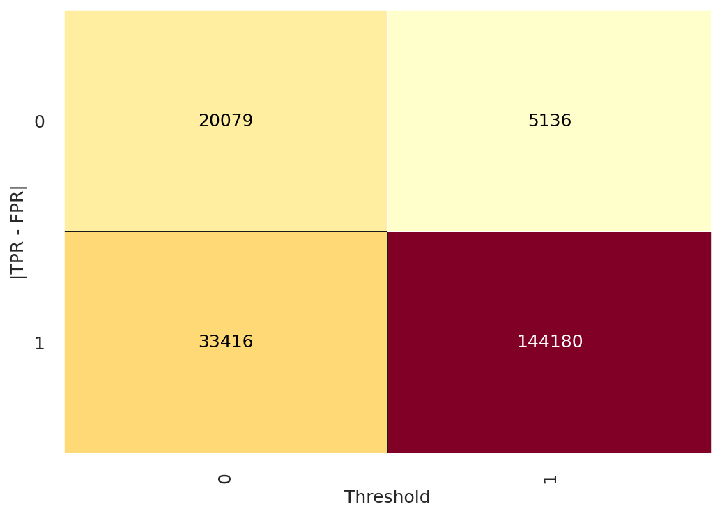
Confusion matrix showing classification performance

ROC Curve

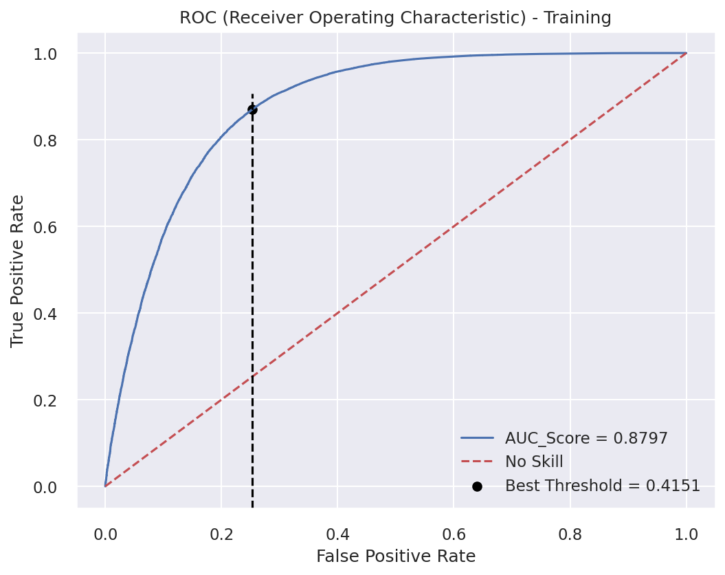
ROC curve showing model discrimination ability

TPR & FPR Analysis

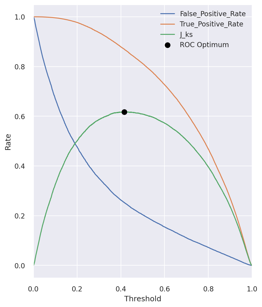
TPR vs FPR at different thresholds

Prediction Distribution Analysis

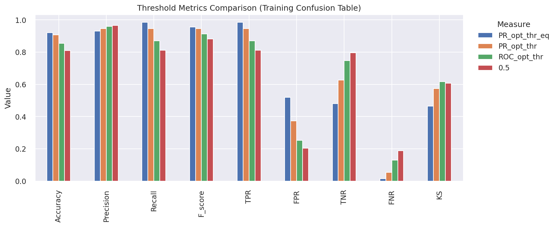
Analysis of predicted probabilities across the dataset, showing how well the model separates good and bad credits.

Performance metrics across different threshold values

Distribution of predicted default probabilities (interactive)

3. Selected Features: Raw Score by Bin Number

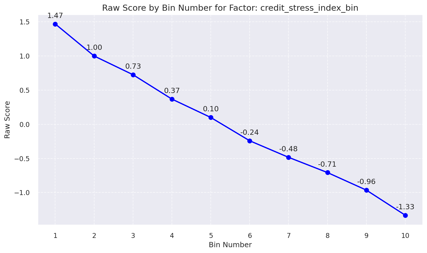
This section visualizes the Weight of Evidence (WOE) scores for selected features, binned by their respective ranges.

Raw Score by Bin: Credit Stress Index Bin

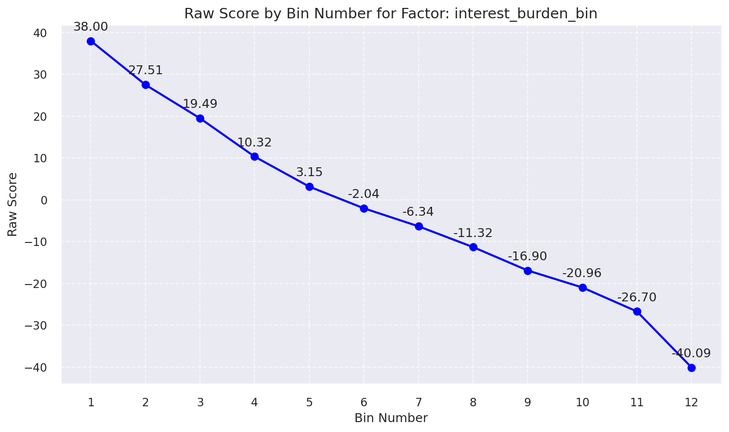
Raw Score by Bin: Interest Burden Bin

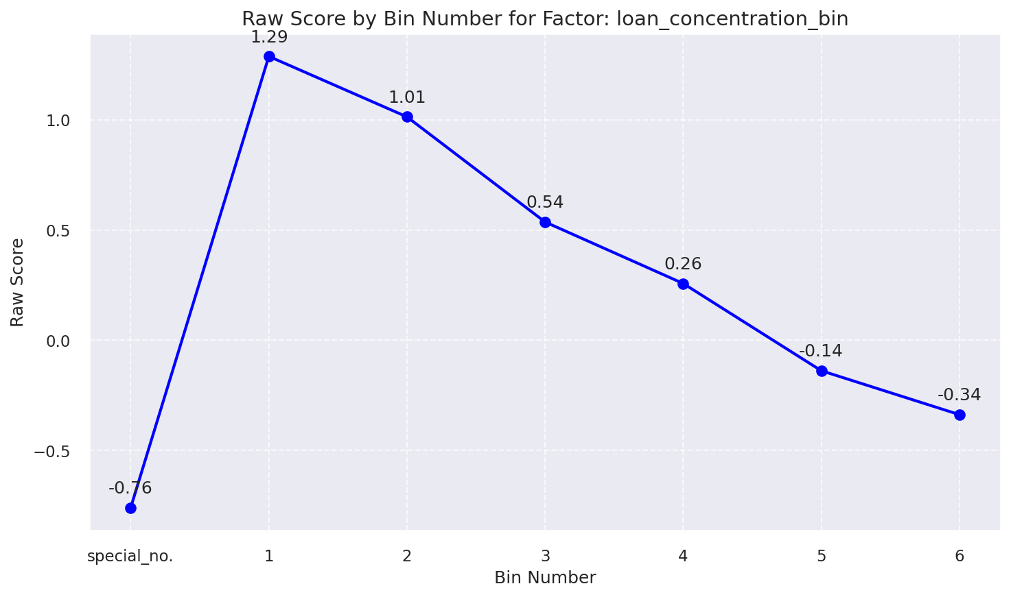
Raw Score by Bin: Loan Concentration Bin

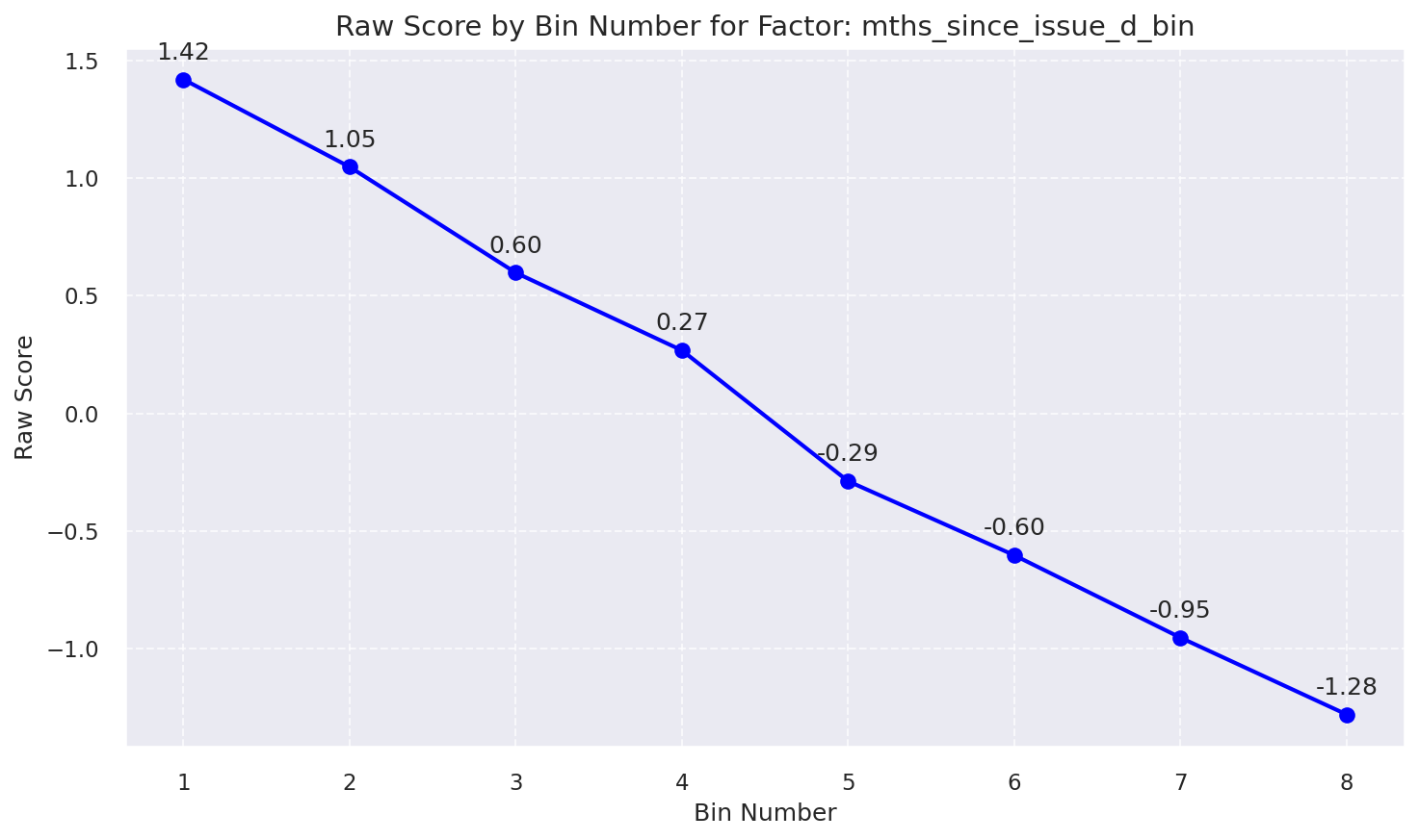
Raw Score by Bin: Mths Since Issue D Bin

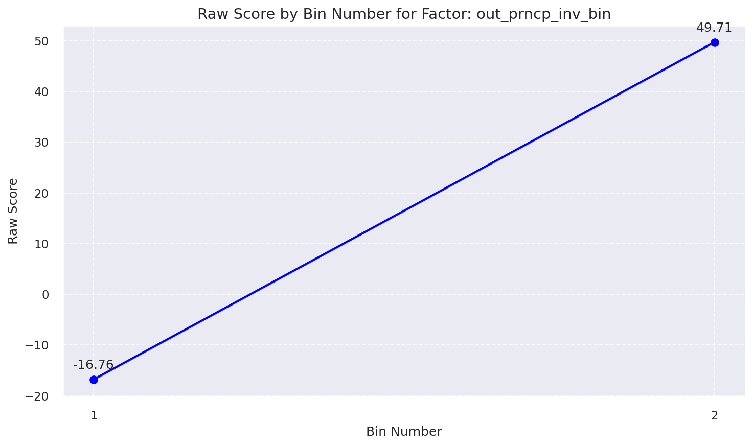
Raw Score by Bin: Out Prncp Inv Bin

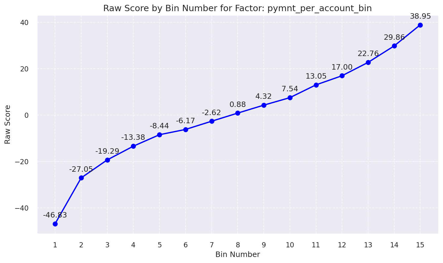
Raw Score by Bin: Pymnt Per Account Bin

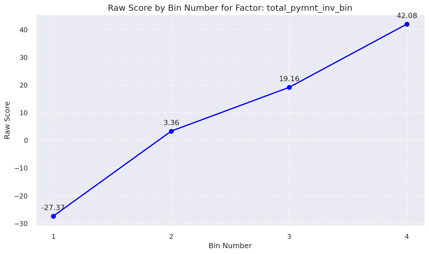
Raw Score by Bin: Total Pymnt Inv Bin

4. Scoring Methods

Comparison of the two scoring methods developed:

Method 1 (WOE Points): Traditional scorecard approach using WOE values and scaling factors.
Method 2 (Probability-to-Score): Direct probability-to-score conversion.

Understanding Percentiles Cut-Off thresholds

These thresholds mean: If my score is greater than the 95th percentile threshold, then my score is greater than 95% of all BAD group scores (I am in the top highest 5%)

Method 1

WOE-based Scorecard

Uses Weight of Evidence (WOE) for each bin to calculate points. The total score is the sum of points plus a base score.

Score = offset + Σ (WOE_bin_i × weight_i × scale)
Or, per-feature breakdown:
Points_i = (WOE_bin_i × weight_i × scale) + (offset / n)
Score = Σ Points_i

Method 2

Probability-based Score

Converts the model's predicted probability of default directly into a credit score.

Probability = logistic(Σ β_i × WOE_i) = 1 / (1 + exp(-(β₀ + Σ β_i × WOE_i)))
Logit = ln(Odds) = ln(Probability / (1 - Probability))
Score = (Factor/ln(2)) × [ln(odds) - ln(baseline_odds)] + Offset

Understanding Score Differences

Understanding Score Differences Between Method 1 and Method 2

Both scoring methods are derived from the same underlying logistic regression model and therefore capture the same latent credit risk signal. The difference between the two approaches lies solely in how the model output is transformed into a final score. Method 1 applies a discretized, bin-based transformation, where fixed points are assigned to predefined WOE bins. Method 2 applies a continuous probability-to-score transformation, converting the model predicted probability of default into a score using a log-odds scaling framework. As a result, the two methods exhibit a very high degree of rank correlation and consistent global risk ordering, while small local differences may occur for observations near bin boundaries due to discretization effects in Method 1. Empirically, this consistency is confirmed by strong Pearson and Spearman correlations between the two score representations.”

Key Point: The risk rank ordering produced by the two methods is highly correlated; in the vast majority of cases, customers assessed as riskier under one method are also assessed as riskier under the other.

Method 1: Bin-Based Scoring

How it works: Assigns fixed points to each WOE bin. Score changes in steps as customers move between bins.

Best For:

Consumer lending decisions (approve/decline)
Adverse action explanations (FCRA/ECOA)
Customer-facing score explanations
Regulatory reporting requiring transparency

Advantage: Maximum transparency — each score component can be directly traced to a specific feature and bin..

Method 2: Probability-Based Scoring

How it works: Converts the predicted probability of default into a continuous credit score using a log-odds transformation.

Best For:

Portfolio risk management & analytics
Expected loss calculations
Risk-based pricing optimization
Basel II / III capital and provisioning frameworks

Advantage: Higher granularity and precision for probability-based risk measurement and threshold optimization.

Regulatory Considerations and Appropriate Use

Important clarification: Both scoring methods are based on a transparent, interpretable logistic regression framework and can be implemented in alignment with applicable regulatory expectations, including Fair Lending principles, FCRA, ECOA, and Basel-related frameworks.

Method 1 is inherently well suited for consumer-facing applications due to its explicit bin-level point attribution and ease of adverse action explanation.
Method 2 is more commonly used for internal risk management, portfolio analytics, and capital planning, where continuous probability estimates are required.
For either method, regulatory compliance is achieved through appropriate implementation, governance, documentation, monitoring, and explanation controls as part of the institution broader model risk management framework, rather than through the scoring transformation alone.<\li> In practice, many mid-to-large financial institutions maintain both score representations concurrently, using the WOE-based scorecard for customer-facing decisions and the probability-based score for internal risk measurement and portfolio optimization.

Recommendation: Use Both Methods

Common industry practice among mid-to-large lenders is to maintain both scoring methods as they serve complementary purposes:

Aspect	Method 1	Method 2
Transparency	⭐⭐⭐⭐⭐	⭐⭐⭐⭐
Granularity	⭐⭐⭐	⭐⭐⭐⭐⭐
Consumer Lending	✅ Preferred	✅ Acceptable
Portfolio Analytics	✅ Acceptable	✅ Preferred

5. Method 1 Results (WOE-Based Scorecard)

Method 1 uses the traditional Weight of Evidence (WOE) approach to calculate credit scores. This method assigns points to each feature based on its WOE value, providing excellent transparency and regulatory compliance. The total score is derived from the sum of individual feature points.

Score Distribution

Interpreting Score Distributions

The score distribution shows how credit scores are spread across good and bad borrowers. A well-performing scorecard should show clear separation between the two groups, with good borrowers having higher scores and bad borrowers having lower scores.

Training Distribution (View 1)

Method 1 score distribution by good/bad credit (training data)

Training Distribution (View 2)

Method 1 score distribution by good/bad credit (training data)

Population Stability Index (PSI)

PSI Interpretation Guidelines

The Population Stability Index (PSI) measures the stability of score distributions over time or across populations:

PSI < 0.1: Stable population - no significant shift detected
PSI 0.1-0.2: Moderate shift - monitor closely for potential model degradation
PSI > 0.2: Significant shift - model recalibration recommended

Training vs Testing

Population Stability Index - Training vs Testing dataset

Observation vs Performance Window

Population Stability Index - Observation vs Performance window

Method 1: Feature Contribution Analysis

Analysis of how each feature contributes to the Method 1 (WOE-based) scoring model.

TOP CONTRIBUTOR

pymnt_per_account

31.80% of total weight

TOTAL SCORE RANGE

552 Points

Sum of all point ranges

TOP 3 FEATURES

76.5%

Combined weight contribution

Feature Score Impact Ranking

Maximum potential score impact (Points Range × Weight%)

Feature Weight = The average of three complementary measures:

IV Weight: Statistical predictive power based on Weight of Evidence bin separation
Point Range: Theoretical maximum score impact points range for this feature
Impact Weight: Model coefficient strength (|Coefficient × WOE|)

pymnt_per_account 48.97

interest_burden 32.00

total_pymnt_inv 27.31

out_prncp_inv 23.35

credit_stress_index 0.07

mths_since_issue_d 0.06

loan_concentration 0.05

📊 Key Insight

pymnt_per_account can swing scores by up to 49 points. Top 3 features account for 108.29 points (82.2% of total scoring power).

Detailed Feature Analysis

Rank	Feature	Points Range	Weight %	Score Impact	Impact Level
1	pymnt_per_account	154.0	31.80%	48.97	Critical
2	interest_burden	140.0	22.86%	32.00	High
3	total_pymnt_inv	125.0	21.85%	27.31	High
4	out_prncp_inv	119.0	19.62%	23.35	High
5	credit_stress_index	5.0	1.31%	0.07	Low
6	mths_since_issue_d	5.0	1.28%	0.06	Low
7	loan_concentration	4.0	1.28%	0.05	Low
TOTAL		552.0	100.00%	131.82

💼 Business Recommendations

✓ Payment Behavior Focus

Payment features drive 53.7% of decisions. Implement early intervention strategies.

✓ Model Monitoring

Track PSI monthly for top 4 features (Score Impact > 10).

✓ Risk Segmentation

Use top 3 features (108 points) for primary risk segmentation.

⚠ Concentration Risk

Top 3 features = 76.5% of weight. Monitor over-reliance.

6. Method 2 Results (Probability-Based Score)

Method 2 converts the model's predicted probability of default directly into a credit score. This approach provides more granular risk assessment and is well-suited for dynamic threshold optimization and portfolio management strategies. The score reflects the model's confidence in the borrower's creditworthiness.

Score Distribution

Score Distribution Characteristics

The probability-based scoring method creates a continuous score distribution that directly reflects the model's risk assessment. Higher scores indicate lower probability of default and vice versa.

Training Distribution (View 1)

Method 2 (Probability-based) score distribution by good/bad credit on training data

Training Distribution (View 2)

Method 2 (Probability-based) score distribution by good/bad credit on training data

Method 2 score comparison across multiple time windows

Population Stability Index (PSI)

PSI Stability Assessment

Monitoring PSI helps ensure the model remains stable over time and across different populations. Consistent low PSI values indicate reliable model performance.

Training vs Testing

Population Stability Index - Training vs Testing dataset

Observation vs Performance Window

Population Stability Index - Observation vs Performance window

7. SHAP Analysis

SHAP (SHapley Additive exPlanations) provides a unified framework for interpreting machine learning models. SHAP values quantify each feature's contribution to individual predictions, offering both global feature importance and local prediction explanations. This analysis helps validate model behavior and ensures decision transparency.

Feature Importance Comparison

Understanding SHAP Values

SHAP values decompose a model's prediction into contributions from each feature. Key insights:

Positive SHAP values: Increase the predicted probability of "good" outcome → indicate lower credit risk
Negative SHAP values: Decrease the predicted probability of "good" outcome → indicate higher credit risk
Magnitude: Indicates the strength of the feature's influence on the prediction
Color coding: Pink/Red = high feature value, Blue = low feature value

SHAP Summary Plots

Class Imbalance Approach 1 (Balanced)

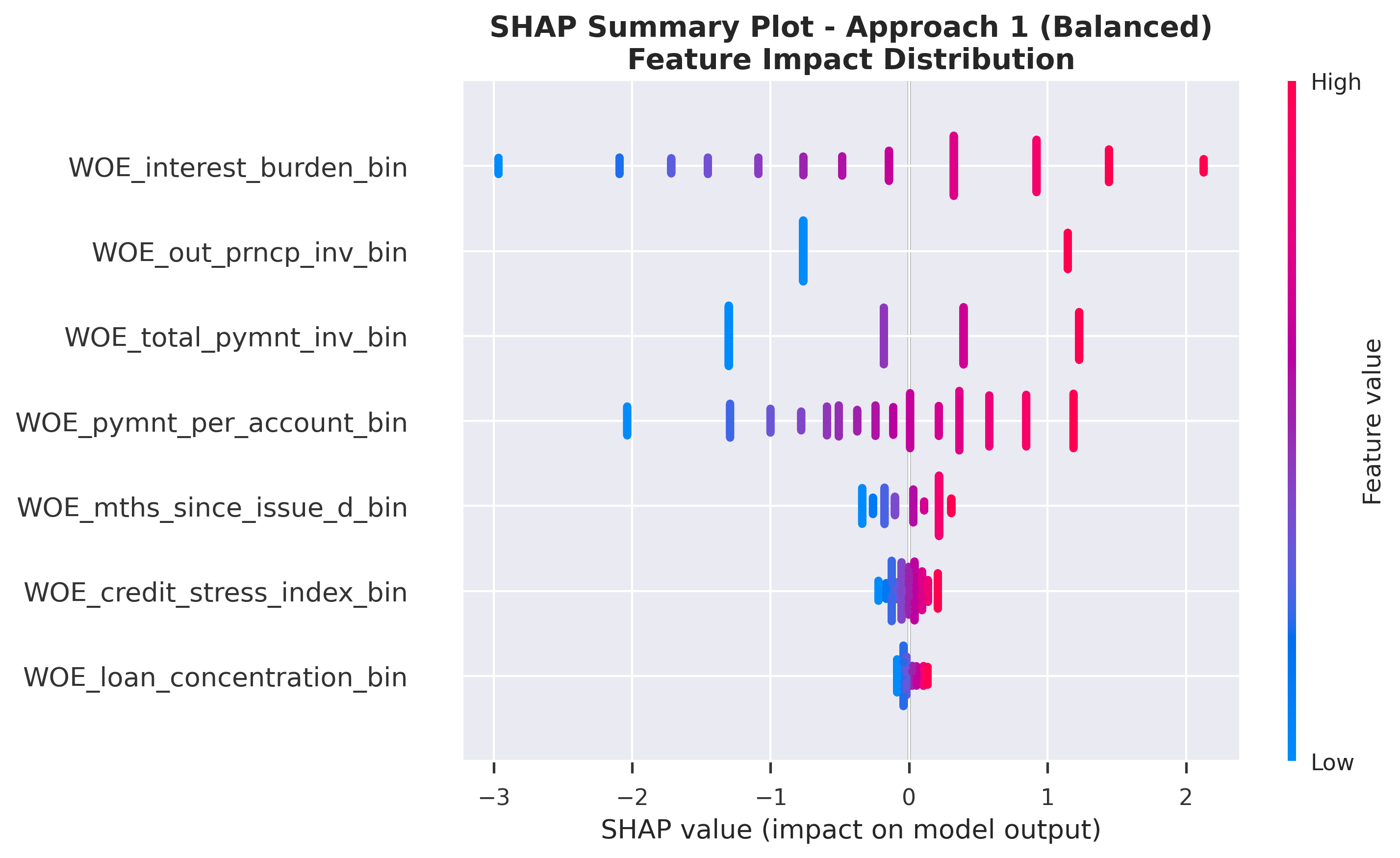
SHAP Feature Impact: Distribution of SHAP values for each feature

Class Imbalance Approach 2 (SMOTE)

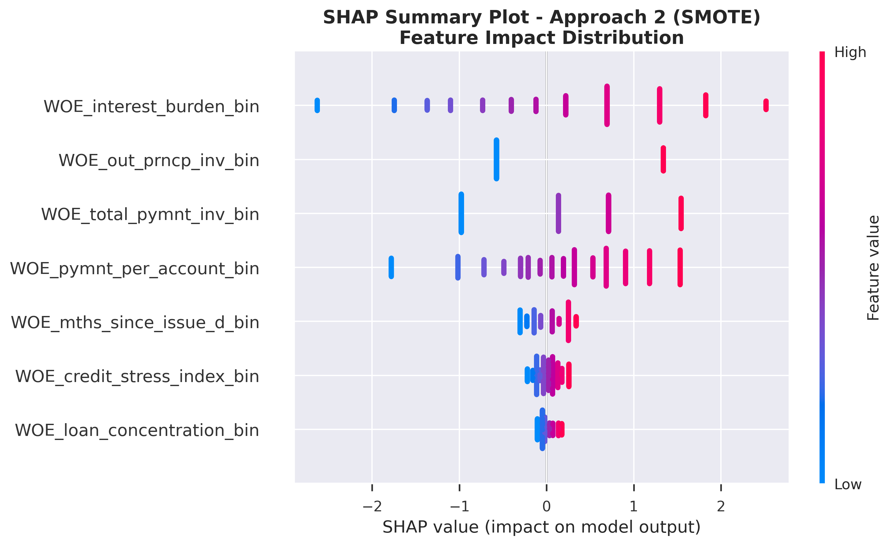
SHAP Feature Impact: Distribution of SHAP values for each feature

SHAP Feature Importance Rankings

Bar plots show mean absolute SHAP values, providing a clear ranking of feature importance. Higher values indicate features with stronger impact on model predictions.

Class Imbalance Approach 1 (Balanced)

Ranked by mean absolute SHAP value

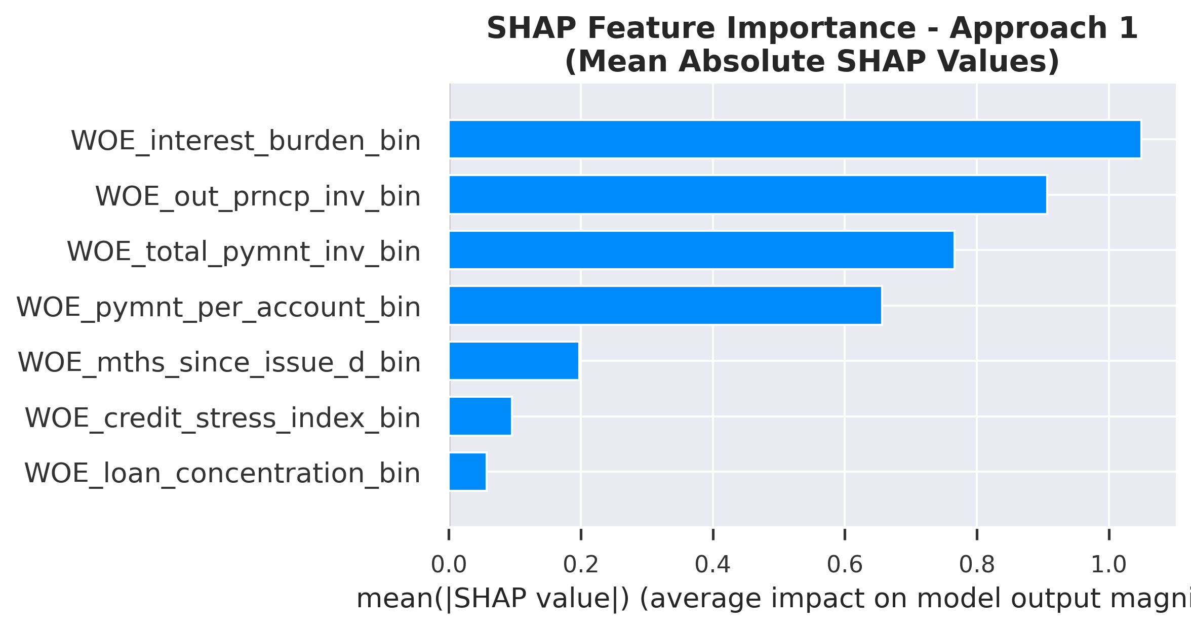
SHAP Feature Importance: Ranked by mean absolute SHAP value

Class Imbalance Approach 2 (SMOTE)

Ranked by mean absolute SHAP value

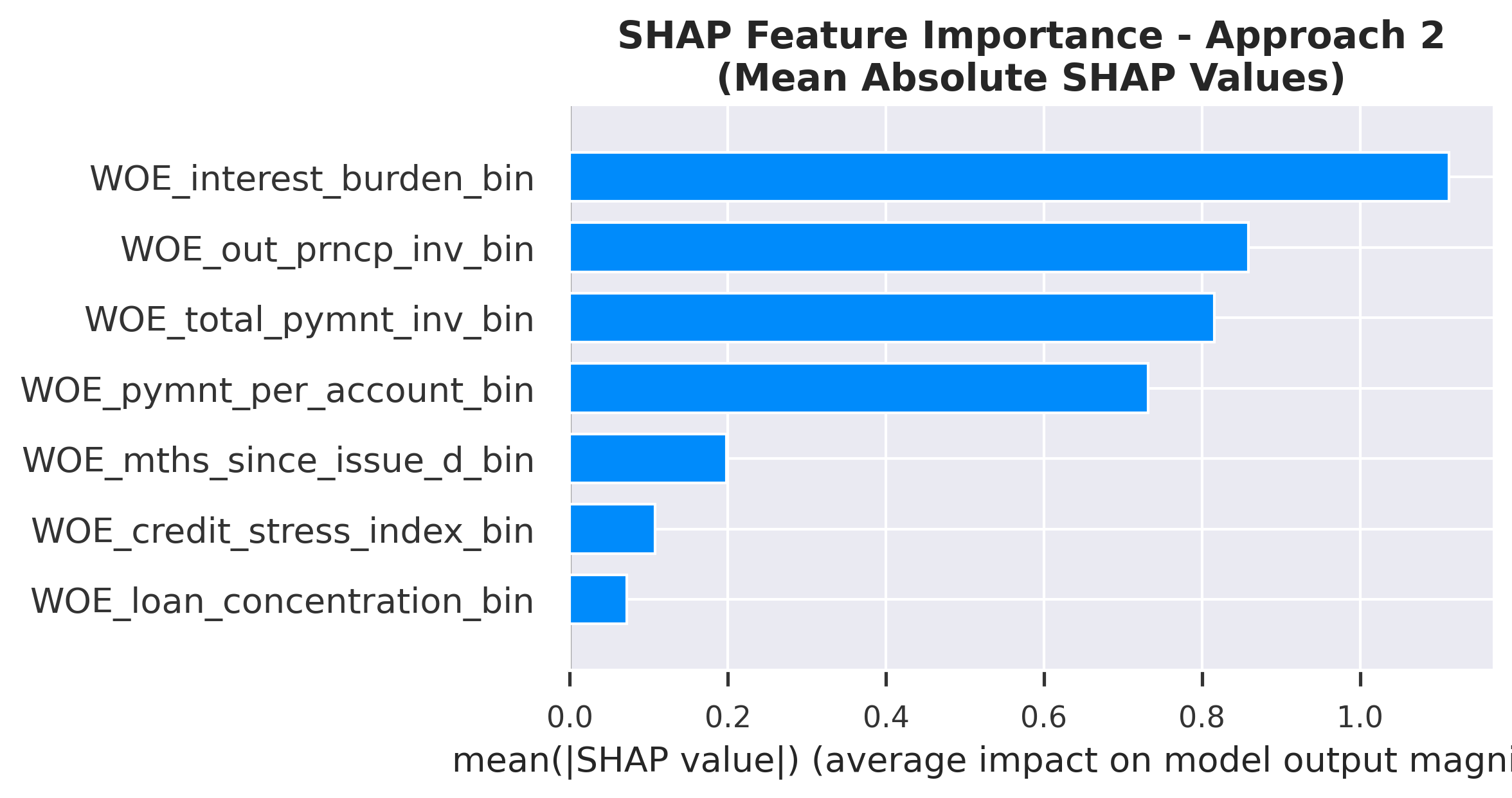
SHAP Feature Importance: Ranked by mean absolute SHAP value

SHAP Feature Importance Comparison

This table compares feature importance across all two approaches using SHAP (SHapley Additive exPlanations) values. Lower rank numbers indicate higher importance. Features are ranked by their mean absolute SHAP value.

Feature	Class Imbalance Approach 1 (Balanced)		Class Imbalance Approach 2 (SMOTE)		Avg Rank
Feature	Rank	Mean \|SHAP\|	Rank	Mean \|SHAP\|	Avg Rank
Interest Burden	1	1.0491	1	1.1125	1.0
Out Prncp Inv	2	0.9067	2	0.8592	2.0
Total Pymnt Inv	3	0.7664	3	0.8157	3.0
Pymnt Per Account	4	0.6567	4	0.7317	4.0
Mths Since Issue D	5	0.1974	5	0.1985	5.0
Credit Stress Index	6	0.0957	6	0.1077	6.0
Loan Concentration	7	0.0574	7	0.0718	7.0

                    Key Insights from Feature Importance
                    Consistent importance: Interest Burden, Out Prncp Inv, Total Pymnt Inv rank
                            as top features across both approaches, indicating they are robust predictors regardless of
                            class balancing method.
Model agreement: Strong agreement (Correlation: 1.00) between Class
                            Imbalance Approaches 1 and 2 rankings confirms that the core risk drivers are stable.
Payment behavior: Payment-related features dominate the top ranks,
                            highlighting that past repayment history is the strongest signal for future default risk.
                        
Stable features: Features like Interest Burden, Out Prncp Inv, Total Pymnt
                            Inv show identical or near-identical rankings, making them highly reliable for policy rules.
                        

                

8. The Two Methods Comparison (WOE-Based Score vs. Probability-Based Score)

This section compares the two scoring methods to assess their distributional characteristics and correlation. Both methods use the same underlying logistic regression model but apply different scaling approaches.

Deviations from Normality (Scores Distribution Q-Q Plot)

Understanding Q-Q Plots

Quantile-Quantile (Q-Q) plots compare the distribution of credit scores against a theoretical normal distribution. Points falling along the diagonal line indicate normality, while deviations suggest the distribution differs from normal. This helps assess whether the scoring methods produce normally distributed scores.

Method 1 (WOE-Based Score)

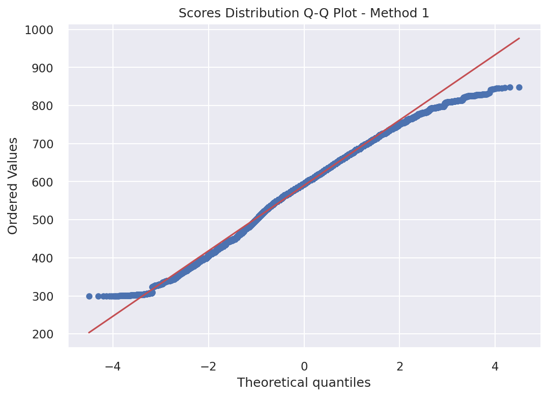
Q-Q Plot for Method 1: Deviation from normality assessment

Method 2 (Probability-Based Score)

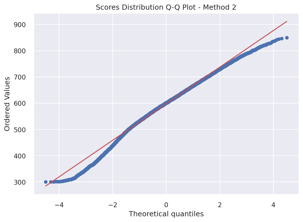
Q-Q Plot for Method 2: Deviation from normality assessment

Score Correlation between the Two Methods

Interpreting Score Correlation

Pearson Correlation: This measures the linear relationship between the two scoring methods.
Spearman Correlation: This measures the monotonic relationship based on ranks rather than actual values.

The correlation plot shows the relationship between scores from Method 1 (WOE-based) and Method 2 (Probability-based). A strong positive correlation indicates that both methods rank customers similarly, even though they use different scales. This validates that both approaches capture the same underlying credit risk.

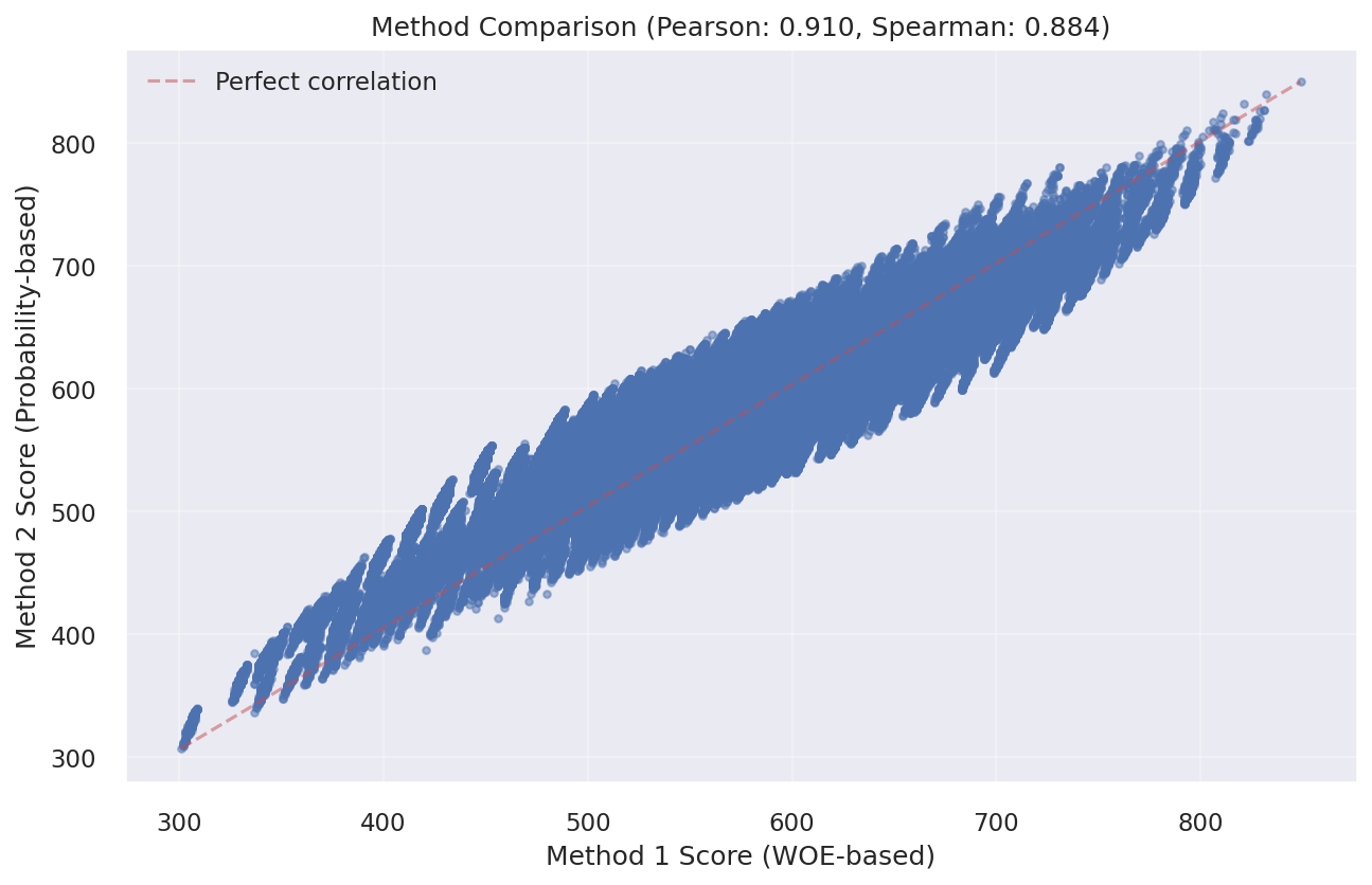
Correlation between Method 1 and Method 2 scores

                    Key Insights from Methods Comparison
                    Distributional Differences: Q-Q plots reveal how each method's score
                            distribution compares to normality
Rank Consistency: High correlation between methods confirms consistent
                            customer ranking despite different scales
Method Selection: Choose Method 1 for regulatory transparency, Method 2 for
                            portfolio analytics
Model Validation: Strong correlation validates that both scoring approaches
                            capture the same risk patterns

                

9. Individual Prediction Explanation

SHAP waterfall plots show how individual features contribute to a specific customer's credit score. Below are example predictions for Customer Index 3 using both scoring methods.

Method 1: WOE-Based Score

Customer Index 3

Score: 538 Points

This score is derived from the sum of WOE-based points across all features. Each feature's WOE value contributes to the final score.

Customer Score Position

Method 1 individual prediction with customer score position (interactive)

Method 2: Probability-Based Score

Customer Index 3

Points: 554 Points

This score is derived from the predicted probability of default. The scoring scale differs from Method 1 but represents the same underlying risk assessment.

Customer Points Position

Method 2 individual prediction with customer points position (interactive)

Feature Contribution Breakdown - For Example Customer Index 3

Waterfall plots explain individual predictions by showing how each feature value pushes the prediction from the baseline (expected value) to the final prediction. Positive SHAP values decrease risk (good), negative values increase risk (bad). This provides transparent, explainable AI for credit decisions.

SHAP Waterfall - Customer Index 3

Total Pymnt Inv Bin

+0.6533

Out Prncp Inv Bin

-0.4682

Mths Since Issue D Bin

-0.2932

Loan Concentration Bin

-0.2928

Credit Stress Index Bin

+0.2777

Pymnt Per Account Bin

-0.2207

Interest Burden Bin

+0.0710

Good Impact

Bad Impact

                    Key Observations
                    Customer Score: Method 1 assigns 538 points, Method 2 assigns 554 points to
                            Customer Index 3
Different Scales: Method 1 and Method 2 use different scoring scales, but
                            both effectively rank credit risk
Interpretability: SHAP values provide transparency into how each feature
                            influences the final prediction
Business Validation: Top features (Total Pymnt Inv, Out Prncp Inv, Mths
                            Since Issue D) align with business intuition

                

10. Credit Risk Tranches Analysis

We segment customers into five distinct tranches based on the Cumulative Distribution Function (CDF) of defaulters. Rather than choosing arbitrary score cutoffs, we use the 10th, 35th, 80th, and 95th percentiles of the historical "bad" population to define our boundaries.

Strategic Tiering

Tranche 1 (0–10th Percentile): Captures the highest concentration of risk. Historically, these represent the bottom 10% of performers and are categorized as Auto-Reject.
Tranche 2 (10th–35th Percentile): Captures the next 25% of the "bad" population. These applications carry significant risk and require Intensive Review.
Tranches 3–5: Segregate the remaining population into Moderate, Low, and Very Low risk tiers.

Methodology Advantage

This methodology ensures that our risk tiers have monotonicity—meaning as you move from one tranche to the next, the probability of default consistently decreases. This provides a data-driven framework for automated decisioning and manual underwriting.

Tranche Interpretation: Tranche labels reflect both individual creditworthiness and portfolio-level default concentration, optimizing for operational risk management rather than absolute probability thresholds.

11. Business Conclusions & Recommendations

Key Risk Drivers Identified

Based on the model's feature importance analysis, the following factors have the highest impact on credit risk prediction:

Interest Burden: High impact on model scoring.
Out Prncp Inv: High impact on model scoring.
Total Pymnt Inv: Strongest indicator of repayment behavior. High impact on model scoring.

Positive Credit Indicators

Features with positive SHAP values (indicating lower default probability):

Note: Most features show mixed directional effects. Refer to SHAP analysis for detailed feature impacts.

Business Recommendations for Lending Teams

Approval Strategy: Use Score threshold of (543+) or (544+) for standard approvals Method1 or Method2, (439.0-549.0) or (475.0-560.0)(Moderate Risk) for manual review with additional documentation Method1 or Method2.
Pricing Optimization: Align interest rates with score bands - lower rates for Exceptional/Very Good, risk-based pricing for Fair/Very Poor.
Portfolio Monitoring: Track PSI monthly; values above 0.1 trigger model review, above 0.2 require recalibration.

Model Comparison Summary

Method 1 (WOE-Based Scorecard): Recommended for regulatory compliance and customer-facing explanations. Each customer's score can be transparently broken down by feature contributions, meeting FCRA and ECOA adverse action requirements.
Method 2 (Probability-to-Score): Recommended for portfolio risk management and dynamic threshold optimization. Provides more granular probability estimates suitable for loss forecasting and capital planning.
Model Stability: Both methods show PSI < 0.1 across test populations, indicating stable model performance over time.